


Figure.1. Exploration Seismology
On this article, I just tried to present some aspect about exploration seismology and visualized by MATLAB, especially a seismic modelling by 2D raytracing in a layered medium and AVO modelling based on synthetic data. It is very pleasant for us of being able to share, to discuss, and to improve our knowledge about geophysical method for oil and gas exploration. Hope at least this little bit will interest us to propose our kind ideas.
Seismic Forward Modelling
The most important technique for exploring oil and gas is to perform the subsurface model of earth’s interior by seismic imaging. “Imaging”, we mean the representation of the earth’s subsurface model. Due to this ultimate goal, geophysicist has imagined seismic forward modelling method by using both numerical study in geoscience and computation technology. Seismic forward modelling will assist us to understand the aspect of seismic traveltime, arrival time, elastic impedance, reflectivity, amplitude that can be generated by seismic energy and the other aspect and it also can be accomplished by ray tracing and synthetic data
.

Seismic Raytracing In a Layered Medium
In a layered medium, the slowness parallel to the interfaces is conserved. Let us first consider a model of homogeneous, plane layers, in the X-Z plane. If the velocity in a i-th layer with thickness ∆Zi , offset ∆Xi is Vi, in this layer we have.

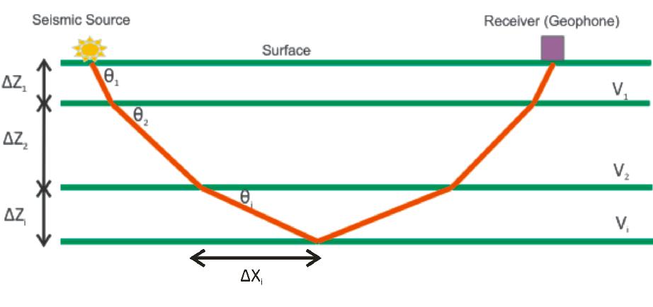

Figure.3. (a). Schematic of raytracing principle through the i-th layer. At each layer the ray is either reflected or transmitted (b). Rays propagate from sources to receivers through flat layers. Red asterisk denotes seismic source, blue box denotes receiver.
Normally we have to be satisfied a unique constant parameter (p) for any particular ray, is commonly called the ray parameter. θi is the angles involved in Snell’s law, can be considered as the angles between the raypaths and the normal to the interface. Up to the critical angle, the raypath intersect at the interface satisfying Snell’s law.

From the geometry of the ray segment in the layer, we can easily calculate the traveltime (T) and how far it goes horizontally to the X axis.


Anyway, Snell’s law is incorporated by replacing the trigonometric functions, so this is similar equation.

Because the medium is a discrete layer, so the summation of ∆Xi refers to the offset of ray will be traveled. In practise, we have to fix it iteratively by using shooting method until any particular ray refers to the receivers position. The summation of ∆Ti refers to total traveltime, also commonly called as two way traveltime (twt).
The offsets are examined by fan of rays and hopefully p values will be found that bracket the desired offset. An alternate approach to finding the intersection is computed iteratively by using bisection technique. If the layer is not flat, we can intersect ray fit to the layer by using spline function, polynomial derivative, interpolation, and line-search method.


Figure.4. (a). Ray diagram for wireline/horizontal survey in a layered medium(b). Seismic traveltime are computed from raytracing


Figure.5. (a). Ray diagram for borehole/vertical seismic profile in a layered medium (b). Seismic traveltime are computed from raytracing
Bisection technique can be applied for solving nonlinear equations like f (x) = 0, only in the case where we know some interval [a, b] on which f (x) is continuous and the solution uniquely exists and, most importantly, f (a) and f (b) have the opposite signs. The procedure toward the solution of f (x) = 0 is described as follows and is cast into MATLAB program.
Amplitude Versus Offset (AVO) Modelling
A variation of reflection and transmission coefficients with incidence angles, and thus offset, is commonly known as amplitude versus offset (AVO). Aki and Richards said that plane-wave reflection and transmission coefficients as a function of incidence angle and elastic properties of the medium. So, to understand AVO is done in order to determine the variations in P-wave (Vp), S-wave (Vs), and density of the medium. It means that changes in sesismic amplitudes with offset are due to contrast in the physical rock properties.
Castagna provided a relationship between Vp and Vs for water-saturated clastic silicate rocks, such as mudstone.

Gardner derived a relationship between density and Vp using empirical observations.

When a plane wave reaches a i-th interface with the particular angle, some of it’s energy is reflected by the boundary and some of its energy is transmitted through the boundary. The portioning of seismic energy is described by the plane wave amplitudes of reflected and transmitted as a function of incidence angle at a i-th interface.
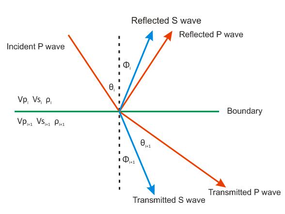
Figure.6. Seismic energy proportion are generated by an incident P-wave through subsurface boundary
Several seismologist has made approximation for plane-wave amplitudes reflection and transmission coefficient. They are Zoeppritz, Shuey, and Thomsen equation. Below, I enclose the PP reflection coefficient which only in a short equation, the complete equations are written in MATLAB function programs.

Figure.7. Raytracing for P-P mode by an incident P-wave in a layered medium

Figure.8. Raytracing for P-S mode by an incident P-wave in a layered medium
Zoeppritz equations are quite complicated and thus their physical meanings are not easily seen. PP and PS reflection coefficient is given below.


Shuey re-wrote the approximation which has been introduced by Aki and Richards in below form. Shuey approximation is fully linearized and more applicable to analyze gradient AVO.

Thomsen approximation is commonly used for various computation to describre the magnitude and the type of rock. His approximation has become the most effective way to compute the portioning of seismic energy at an interface. PP reflection coefficient is given below.

Synthetic Test For P-P & P-S Reflection
For proper analyze, we also need to examine the variation of amplitude as changes of incidence angle. The AVO as seismic response generate from the synthetic data, such as elastic parameter, geology model, and spatial geometry of the source-receiver offsets configuration. Below, I tried to make a simple lithology of 13 layers, including model of P wave velocity, S wave velocity, and density. Seismic reflection geometry is designed from 0 to 2000 metres and covers 2000 metres of maximum depth. Receiver interval 20 metres, 3 shot positions at 0 m, 1000 m, and 2000 m along the surface of geometry setting.

Figure.9. Lithology model of P wave velocity, S wave velocity, and density
Lithology model, geometry experiment, source-receiver configuration, and cross plots are figured by Matlab program (model.m), raytracing process are computed by shooting.m (modified from CREWES program), Reflection coefficient Rpp and Rps are calculated by zoeppritz.m, shuey.m, and thomsen.m, synthetic log for P sonic, S sonic, and density log are estimated by logsyn.m. For study purpose, I enclose Matlab program and it is recomended to modify all source codes if there were wrong algorithms.

Figure.10. Raytracing P-P mode by an incident P-wave in a layered medium of seismic reflection experiment.

Figure.11. Raytracing P-S mode by an incident P-wave in a layered medium of seismic reflection experiment

Figure.12. Stacked section of seimogram synthetic for P-P reflection coefficient after convolving with 20 Hz ricker wavelet.

Figure.13. Stacked section of seimogram synthetic for P-S reflection coefficient after convolving with 20 Hz ricker wavelet

Figure.14. Stacked section of seimogram synthetic for both P-P and P-S reflection coefficient after convolving with 20 Hz ricker wavelet

Figure.15. Comparison of approximation between exact reflection coefficients versus absolut incidence angle from lithology model

Figure.16.(a). Cross plot of intercept vs gradient AVO from the lithology model, (b). Cross plot of reflection coefficient vs sine square of angles.
Synthetic Log & Seismogram
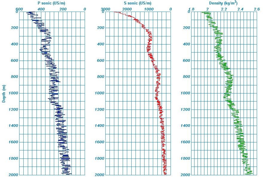
Figure.17 P sonic, S Sonic, and density log (synthetic) from the lithology model

Figure.18 Cross plot of physical rock properties from the lithology model

Figure.19. (a). Poisson ratio, (b). Synthetic seismogram after convolving with 20 Hz ricker wavelet, (c). Stacked section of PP seimic traces from AVO modelling
Further, the results are useful in applying seismic inversion, to get better approximation of actual geology, and also to analyze the physical rock properties in petroleum systems. The majority of oil and gas industry have initiated and still develop their seismic imaging methodology. Be able to characterize accurately the reservoirs that are associated with paradox formation or complex geology is not pure easily applied. As prior, we have to do low-cost investigation before drilling by using sophisticated tools. Usually an extensive and successful drilling program has been conducted by forwarding the best seismic imaging.

Marine seismic data acquisition (From Schlumberger, 1990)

However, either exploration or exploitation of hydrocarbon is not just a journey to employ people, upgrading tools, allocating budget to support acquiring the data, extensive drilling, and the other supporting activities. Naturally, resources and disaster or accident are illustrated as two sides of coin. Always becoming most important notice to consider the aspect of environmental and social sensitivity, safety, energy saving, reduction poverty and prosperity of life.
References :
Carcuz, J.R., 2001, A combined AVO analysis of P-P and P-S reflection data: SEG Expanded Abstracts 20,323-325.
MATLAB SOURCE CODES (model.m)
% model.m
%==========================================================================================
% MAIN PROGRAM
%==========================================================================================
clc; clear all; close all;
format short g
%============================================================================================
% Define Geometry
%============================================================================================
fprintf('---> Defining the interfaces ...\n');
% Input geometry
xmin = 0; xmax = 2000;
zmin = 0; zmax = 2000;
% Make strata layer
zlayer = [0;80;180;300;450;630;800;1050;1200;1400;1620;1820;2000];
nlayer = length(zlayer);
layer = 1:1:nlayer;
thick = abs(diff(zlayer));
x = [xmin xmax]; z = [zlayer zlayer];
dg = 10;
xx = xmin:dg:xmax; nx = length(xx);
zz = repmat(zlayer,1,nx);
fprintf(' Geometry has been defined...[OK]\n');
%============================================================================================
% Source-Receiver Groups
%============================================================================================
fprintf('---> Setting source-receiver configuration ...\n');
% Receiver Interval
dr = 20;
% Mix Configuration
% Source
% xs = [55 1350];
% zs = [0 690];
% ns = length(xs);
%
% % Receiver
% xr = [200 500 850 1600 1900];
% zr = [300 0 220 150 0];
% nr = length(xr);
% --------------------------------------
% Front Configuration
% Source
% xs = xmin;
% zs = 0;
% ns = length(xs);
%
% % Receiver
% xr = xmin+dr:dr:xmax;
% zr = zeros(length(xr));
% nr = length(xr);
% --------------------------------------
% End Configuration
% Source
% xs = xmax;
% zs = 0;
% ns = length(xs);
%
% % Receiver
% xr = xmax-dr:-dr:xmin;
% zr = zeros(length(xr));
% nr = length(xr);
% --------------------------------------
% Split Spread Configuration
% Source
% xs = fix((xmax-xmin)/2);
% zs = 0;
% ns = length(xs);
%
% % Receiver
% xr = [fix((xmax-xmin)/2)-dr:-dr:xmin fix((xmax-xmin)/2)+dr:dr:xmax];
% zr = zeros(length(xr));
% nr = length(xr);
% --------------------------------------
% Off-End Configuration
% Source
% xs = [xmin xmax];
% zs = [0 0];
% ns = length(xs);
%
% % Receiver
% xr = xmin+dr:dr:xmax-dr;
% zr = zeros(length(xr));
% nr = length(xr);
% Front Spread Configuration
% Source
xs = [xmin fix((xmax-xmin)/2) xmax];
zs = [0 0 0];
ns = length(xs);
% Receiver
xr = [xmin+dr:dr:fix((xmax-xmin)/2)-dr fix((xmax-xmin)/2)+dr:dr:xmax-dr];
zr = zeros(length(xr));
nr = length(xr);
% VSP Configuration
% Source
% xs = 1950;
% zs = 0;
% ns = length(xs);
%
% % Receiver
% zr = 0:100:1600;
% xr = 50.*ones(length(zr));
% nr = length(xr);
nray = ns*nr;
fprintf(' Source-Receiver Groups have been setted...[OK]\n');
%============================================================================================
% Create Elastic Parameter
%============================================================================================
fprintf('---> Creating elastic parameter ...\n');
% Create synthetic Vp, Vs, and Density
vlayer = [1800;2000;2200;2500;2400;2700;3150;2950;3440;3750;4000;4350;4600]; % Velocity
vlayer = vlayer(1:length(zlayer));
vel = [vlayer vlayer];
vp = vlayer; % P wave velocity
vs = (vp-1360)./1.16; % S wave velocity based on Castagna's rule
ro = 0.31.*(vp).^0.25; % Density based on Gardner's rule
pois = (vs.^2-0.5*vp.^2)./(vs.^2-vp.^2); % Poisson ratio
fprintf(' No.Layer Depth(m) Vp(m/s) Vs(m/s) Density(kg/m^3) Poisson Ratio \n');
disp([layer' zlayer vp vs ro pois]);
fprintf(' Elastic parameters have been created...[OK]\n');
figure;
set(gcf,'color','white');
% Plot P wave velocity
subplot(1,3,1);
stairs(vp,zlayer,'LineWidth',2.5,'Color',[0.07843 0.1686 0.549]);
ylabel('Depth (m)','FontWeight','bold','Color','black');
title('V_{p} (m/s)','FontWeight','bold');
set(gca,'XMinorGrid','on','YMinorGrid','on','YDir','reverse','YColor',[0.04314 0.5176 0.7804],...
'XAxisLocation','top','XColor',[0.04314 0.5176 0.7804],'MinorGridLineStyle','-','FontWeight',...
'demi','FontAngle','italic');
% Plot S wave velocity
subplot(1,3,2);
stairs(vs,zlayer,'LineWidth',2.5,'Color',[1 0 0]);
title('V_{s} (m/s)','FontWeight','bold');
set(gca,'XMinorGrid','on','YMinorGrid','on','YDir','reverse','YColor',[0.04314 0.5176 0.7804],...
'XAxisLocation','top','XColor',[0.04314 0.5176 0.7804],'MinorGridLineStyle','-','FontWeight',...
'demi','FontAngle','italic');
% Plot Density
subplot(1,3,3);
stairs(ro,zlayer,'LineWidth',2.5,'Color',[0.07059 0.6392 0.07059]);
title('Density (kg/m^3)','FontWeight','bold');
set(gca,'XMinorGrid','on','YMinorGrid','on','YDir','reverse','YColor',[0.04314 0.5176 0.7804],...
'XAxisLocation','top','XColor',[0.04314 0.5176 0.7804],'MinorGridLineStyle','-','FontWeight',...
'demi','FontAngle','italic');
% Plot Geology Model
figure;
set(gcf,'color','white');
color = load('mycmap.txt');
pcolor(xx,zz,repmat(vlayer,1,nx)); shading flat; hold on
colormap(color); colorbar ('horz');
axis([0 xmax zmin-0.03*zmax zmax])
set(gca,'YDir','reverse','XaxisLocation','bottom',....
'Ytick',zlayer,'FontWeight','demi','PlotBoxAspectRatioMode','Manual',...
'PlotBoxAspectRatio',[2.4 1.2 1],'Position',[0.04 0.30 0.90 0.60]);
% Plot Source-Receiver Group
plot(xs,zs,'r*','markersize',12); hold on
plot(xr,zr,'sk','markersize',4,'markerfacecolor','c'); hold on
xlabel('Velocity (m/s)','FontWeight','bold','Color','black');
ylabel('Depth (m)','FontWeight','bold','Color','black');
%============================================================================================
% Run Ray Tracing
%============================================================================================
fprintf('---> Starting ray tracing ...\n');
wat = waitbar(0,'Raytracing is being processed, please wait...');
%============================================================================================
xoff = [];
% Loop over for number of souce
tic
for i=1:ns
% Loop over for number of receiver
for j=1:nr
%====================================================================================
% Loop over for number of layer
for k=1:nlayer
%=====================================================================================
% Declare reflection boundary
if and(zr(j) < zlayer(k),zs(i) < zlayer(k))
zm = zz(k,:); zf = min(zm)- 100000*eps;
% Downgoing path
d = find(zlayer > zs(i));
if(isempty(d)); sdown = length(zlayer); else sdown = d(1)-1; end
d = find(zlayer > zf);
if(isempty(d)); edown = length(zlayer); else edown = d(1)-1; end
zd = [zs(i);zlayer(sdown+1:edown)]; nd = length(zd);
% Upgoing path
u = find(zlayer > zr(j));
if(isempty(u)); sup = length(zlayer); else sup = u(1)-1; end
u = find(zlayer > zf);
if(isempty(u)); eup = length(zlayer); else eup = u(1)-1; end
zu = [zr(j);zlayer(sup+1:eup+1)]; nu = length(zu);
zn = [zd;(flipud(zu))]; nrefl = length(zn)-1;
%=================================================================================
% Declare elastic parameter
% Downgoing elastic parameter
vpd = [vp(sdown:edown);vp(edown)];
vsd = [vs(sdown:edown);vs(edown)];
rod = [ro(sdown:edown);ro(edown)];
% Upgoing elastic parameter
vpu = [vp(sup:eup);vp(eup)];
vsu = [vs(sup:eup);vs(eup)];
rou = [ro(sup:eup);ro(eup)];
% Combine model elastic parameter
vpp = [vpd(1:end-1);flipud(vpu(1:end-1))];
vss = [vsd(1:end-1);flipud(vsu(1:end-1))];
vps = [vpd(1:end-1);flipud(vsu(1:end-1))];
rho = [rod(1:end-1);flipud(rou(1:end-1))];
%=================================================================================
% Start Raytracing (P-P, S-S, or P-S mode)
ops = 1; % ops=1 for PP mode; ops=2 for PS mode
[xh,zh,vh,pp,teta,time] = shooting(vpp,vps,zn,xx,xs(i),xr(j),ops);
theta = abs(teta); twt(k,j,i) = time;
% Plot Ray
if ops == 1
plot(xh,zh,'k-');
title('Seismic Raytracing (P-P mode)','FontWeight','bold');
elseif ops == 2
xd = xh(1:nd+1); xu = xh(nd+1:end);
zd = zh(1:nd+1); zu = zh(nd+1:end);
plot(xd,zd,'k-',xu,zu,'r-');
title('Seismic Raytracing (P-S mode)','FontWeight','bold');
end
%=================================================================================
% Compute Reflection Coefficient (Downgoing-Upgoing)
for c=1:nrefl-1
% Reflection Coefficient of Zoeppritz Approximation
[rc1,teta] = zoeppritz(pp,theta(c),vpp(c),vss(c),rho(c),theta(c+1),...
vpp(c+1),vss(c+1),rho(c+1),ops);
rcz(c,j,i) = rc1;
% Reflection Coefficient of Shuey Approximation
[A,B,rc2,teta] = shuey(theta(c),vpp(c),vss(c),rho(c),theta(c+1),...
vpp(c+1),vss(c+1),rho(c+1),ops);
rcs(c,j,i) = rc2; AA(c,j,i) = A; BB(c,j,i) = B;
% Reflection Coefficient of Thomsen Approximation
[rc3,teta] = thomsen(theta(c),vpp(c),vss(c),rho(c),theta(c+1),...
vpp(c+1),vss(c+1),rho(c+1));
rct(c,j,i) = rc3;
angle(c,j,i) = teta.*(180/pi);
end
%====================================================================================
end
end % for horizon/reflector end
xoff = [xoff xr(j)];
waitbar(j/nray,wat)
end % for receiver end
% Save Data
save(['time_shot',num2str(i),'.mat'],'twt');
save(['reflz_shot',num2str(i),'.mat'],'rcz');
save(['refls_shot',num2str(i),'.mat'],'rcs');
save(['reflt_shot',num2str(i),'.mat'],'rct');
save(['teta_shot',num2str(i),'.mat'],'angle');
save(['intercept_shot',num2str(i),'.mat'],'AA');
save(['gradient_shot',num2str(i),'.mat'],'BB');
waitbar(i/ns,wat)
end % for sources end
%=============================================================================================
close(wat);
toc
fprintf(' Ray tracing has succesfully finished...[OK]\n');
xx = repmat(xr,nlayer,1);
% Plot Traveltime
figure;
for i=1:ns
tm = load(['time_shot',num2str(i),'.mat']); tt = tm.twt;
plot(xx(2:nlayer,:),tt(2:nlayer,:,i),'b.'); hold on
xlabel('Horizontal Position (m)','FontWeight','bold','FontAngle','normal','Color','black');
ylabel('Time (s)','FontWeight','bold','FontAngle','normal','Color','black');
title('Traveltime','FontWeight','bold');
set(gca,'Ydir','reverse');
set(gcf,'color','white');
end
% Plot Reflection Coefficient
figure;
for i=1:ns
reflz = load(['reflz_shot',num2str(i),'.mat']); reflz = reflz.rcz;
refls = load(['refls_shot',num2str(i),'.mat']); refls = refls.rcs;
reflt = load(['reflt_shot',num2str(i),'.mat']); reflt = reflt.rct;
theta = load(['teta_shot',num2str(i),'.mat']); angle = theta.angle;
%Reflection Coefficient of Zoeppritz
subplot(1,3,1)
plot(abs(angle(1:nlayer,:,i)),reflz(1:nlayer,:,i),'r.'); hold on
xlabel('Incidence Angles (degree)','FontWeight','bold','Color','black');
ylabel('Reflection Coefficient','FontWeight','bold','Color','black');
grid on; title('Rpp Zoeppritz','FontWeight','bold','Color','black')
set(gca,'YColor',[0.04314 0.5176 0.7804],'XColor',[0.04314 0.5176 0.7804]); hold on
%Reflection Coefficient of Shuey
subplot(1,3,2)
plot(abs(angle(1:nlayer,:,i)),refls(1:nlayer,:,i),'g.'); hold on
xlabel('Incidence Angles (degree)','FontWeight','bold','Color','black');
grid on; title('Rpp Shuey','FontWeight','bold','Color','black')
set(gca,'YColor',[0.04314 0.5176 0.7804],'XColor',[0.04314 0.5176 0.7804]); hold on
%Reflection Coefficient of Thomsen
subplot(1,3,3)
plot(abs(angle(1:nlayer,:,i)),reflt(1:nlayer,:,i),'b.'); hold on
xlabel('Incidence Angles (degree)','FontWeight','bold','Color','black');
grid on; title('Rpp Thomsen','FontWeight','bold','Color','black')
set(gca,'YColor',[0.04314 0.5176 0.7804],'XColor',[0.04314 0.5176 0.7804]); hold on
set(gcf,'color','white');
end
for i=1:ns
refls = load(['refls_shot',num2str(i),'.mat']); refls = refls.rcs;
theta = load(['teta_shot',num2str(i),'.mat']); angle = theta.angle;
Rt = load(['intercept_shot',num2str(i),'.mat']); Rt = Rt.AA;
Gt = load(['gradient_shot',num2str(i),'.mat']); Gt = Gt.BB;
Ro(1:nlayer,:,i) = Rt(1:nlayer,:,i);
Go(1:nlayer,:,i) = Gt(1:nlayer,:,i);
Rc(1:nlayer,:,i) = refls(1:nlayer,:,i);
inc(1:nlayer,:,i) = angle(1:nlayer,:,i);
end
Rp = reshape(Ro,nr*ns*nlayer,1);
G = reshape(Go,nr*ns*nlayer,1);
R = reshape(Rc,nr*ns*nlayer,1);
teta = reshape(inc,nr*ns*nlayer,1);
% Plot Attributes
figure;
% Rp-G Cross Plot
subplot(1,2,1)
plot(Rp,G,'r.'); hold on
plot(Rl,G,'m-'); hold on
xlabel('R','FontWeight','bold','Color','black');
ylabel('G','FontWeight','bold','Color','black');
grid on; title('R-G Cross Plot','FontWeight','bold','Color','black')
set(gca,'YColor',[0.04314 0.5176 0.7804],'XColor',[0.04314 0.5176 0.7804]); hold on
% R-sin^2(teta) Cross Plot
subplot(1,2,2)
plot((sin(teta).^2),R,'g.'); hold on
xlabel('sin^2(teta)','FontWeight','bold','Color','black');
ylabel('R(teta)','FontWeight','bold','Color','black');
grid on; title('R-sin^2(teta) Cross Plot','FontWeight','bold','Color','black')
set(gca,'YColor',[0.04314 0.5176 0.7804],'XColor',[0.04314 0.5176 0.7804]); hold on
set(gcf,'color','white');
%============================================================================================
% AVO Modelling
%============================================================================================
fprintf('---> Starting AVO Modelling ...\n');
% Make wavelet ricker (f = 2 Hz)
dt = 0.004; f = 20;
[w,tw] = ricker(dt,f);
% Create zeros matrix for spike's location
tmax = max(tt(:));
tr = 0:dt:tmax; nt = length(tr);
t = tt(2:nlayer,:);
% Take reflectivity into spike location
spikes = zeros(nt,nray);
rcz = real(reflz(2:nlayer,:));
for k=1:nlayer-1
for j=1:nray
ir(k,j) = fix(t(k,j)/dt+0.1)+1;
spikes(ir(k,j),j) = spikes(ir(k,j),j) + rcz(k,j);
end
end
% Convolve spikes with wavelet ricker
for j=1:nray
seisz(:,j) = convz(spikes(:,j),w);
end
ampz=reshape(seisz,length(tr),nr,ns);
for i=1:ns
ampz_shot(:,:,i) = ampz(:,:,i);
save(['ampz_shot',num2str(i),'.mat'],'ampz_shot');
end
% CMP Stacked
Stacked = zeros(nt,nr);
for i=1:ns
files = load(['ampz_shot',num2str(i),'.mat']);
files = files.ampz_shot;
Stacked = Stacked + files(:,:,i);
end
% Save Seismic Data
save(['seis','.mat'],'Stacked');
% Plot AVO
figure;
wig(xr,tr,Stacked,'black'); hold on
xlabel('Offset (m)','FontWeight','bold','Color','black');
ylabel('Time (s)','FontWeight','bold','Color','black');
title('Synthetic Seismogram','FontWeight','bold','Color','black');
axis tight
set(gca,'YColor',[0.04314 0.5176 0.7804],'XColor',[0.04314 0.5176 0.7804]); hold on
set(gcf,'color','white');
fprintf(' AVO Modelling has been computed...[OK]\n');
%============================================================================================
% Seismogram Synthetic
%============================================================================================
% Create Smooth Synthetic Log From Elastic Data Set
[pson,sson,spson,rlog,zlog] = logsyn(vp,vs,ro,zlayer,500);
vplog = 1.0e6./pson; vslog = 1.0e6./sson;
rholog = 0.31.*(vplog).^0.25; vpvs = vplog./vslog;
poisson = (vslog.^2-0.5*vplog.^2)./(vslog.^2-vplog.^2);
% Plot Synthetic Data Log
figure;
set(gcf,'color','white');
% Plot P Sonic Log
subplot(1,3,1);
stairs(pson,zlog,'LineWidth',1,'Color',[0.07843 0.1686 0.549]);
xlabel('P sonic (US/m)','FontWeight','bold','Color','black');
ylabel('Depth (m)','FontWeight','bold','Color','black');
set(gca,'XMinorGrid','on','YMinorGrid','on','YDir','reverse','XDir','reverse','YColor',...[0.04314 0.5176 0.7804],'XAxisLocation','top','XColor',...
[0.04314 0.5176 0.7804],'MinorGridLineStyle','-','FontWeight','demi','FontAngle','italic');
% Plot S Sonic Log
subplot(1,3,2);
stairs(sson,zlog,'LineWidth',1,'Color',[1 0 0]);
xlabel('S sonic (US/m)','FontWeight','bold','Color','black');
set(gca,'XMinorGrid','on','YMinorGrid','on','YDir','reverse','XDir','reverse','YColor',[0.04314 0.5176 0.7804],...
'XAxisLocation','top','XColor',[0.04314 0.5176 0.7804],'MinorGridLineStyle','-','FontWeight',...
'demi','FontAngle','italic');
% Plot Density Log
subplot(1,3,3);
stairs(rlog,zlog,'LineWidth',1,'Color',[0.07059 0.6392 0.07059]);
xlabel('Density (kg/m^3)','FontWeight','bold','Color','black');
set(gca,'XMinorGrid','on','YMinorGrid','on','YDir','reverse','YColor',[0.04314 0.5176 0.7804],...
'XAxisLocation','top','XColor',[0.04314 0.5176 0.7804],'MinorGridLineStyle','-','FontWeight',...
'demi','FontAngle','italic');
% Plot Rock Properties
figure;
% Cross Plot P and S wave velocity
subplot(2,2,1);
plot(vplog,vslog,'.','Color',[0.07843 0.1686 0.549]);
xlabel('Vp (m/s)','FontWeight','bold','Color','black');
ylabel('Vs (m/s)','FontWeight','bold','Color','black');
title('Cross Plot of Vp and Vs','FontWeight','bold','Color','black');
set(gca,'XMinorGrid','on','YMinorGrid','on','YColor',[0.04314 0.5176 0.7804],...
'XAxisLocation','bottom','XColor',[0.04314 0.5176 0.7804],'MinorGridLineStyle',...
'-','FontWeight','demi','FontAngle','italic');
% Plot S Sonic Log
subplot(2,2,2);
plot(vplog,vpvs,'.','Color',[1 0 0]);
xlabel('Vp (m/s)','FontWeight','bold','Color','black');
ylabel('Vp/Vs ratio','FontWeight','bold','Color','black');
title('Cross Plot of Vp and Vp/Vs Ratio','FontWeight','bold','Color','black');
set(gca,'XMinorGrid','on','YMinorGrid','on','YColor',[0.04314 0.5176 0.7804],...
'XAxisLocation','bottom','XColor',[0.04314 0.5176 0.7804],...
'MinorGridLineStyle','','FontWeight',...
'demi','FontAngle','italic');
% Plot Density Log
subplot(2,2,3);
plot(rholog,vpvs,'.','Color',[0.07059 0.6392 0.07059]);
xlabel('Density (kg/m^3)','FontWeight','bold','Color','black');
ylabel('Vp/Vs ratio','FontWeight','bold','Color','black');
title('Cross Plot of Vp and Vp/Vs Ratio','FontWeight','bold','Color','black');
set(gca,'XMinorGrid','on','YMinorGrid','on','YColor',[0.04314 0.5176 0.7804],...
'XAxisLocation','bottom','XColor',[0.04314 0.5176 0.7804],'MinorGridLineStyle',...
'-','FontWeight','demi','FontAngle','italic');
subplot(2,2,4);
plot(poisson,vpvs,'m.');
xlabel('Poisson Ratio','FontWeight','bold','Color','black');
ylabel('Vp/Vs ratio','FontWeight','bold','Color','black');
title('Cross Plot of Vp and Vp/Vs Ratio','FontWeight','bold','Color','black');
set(gca,'XMinorGrid','on','YMinorGrid','on','YColor',[0.04314 0.5176 0.7804],...
'XAxisLocation','bottom','XColor',[0.04314 0.5176 0.7804],'MinorGridLineStyle',...
'-','FontWeight','demi','FontAngle','italic');
set(gcf,'color','white');
% Integrate Depth and Velocity To Get Two-Way Time
tstart = 0; tracenum = 10;
[tz,zt] = sonic2tz(spson,zlog,-100,tstart);
tzobj = [zt tz];
vins = vplog; dens = rholog; z = zlog;
% Determine Ricker Wavelet
dt = 0.004; f = 20;
[w,tw] = ricker(dt,f);
[theo,tlog,rcs,pm,p] = seismogram(vins,dens,z',w,tw,tzobj,0,0,1);
% Convolves Reflectivity With Wavelet
nint = length(tlog);
RC = zeros(length(tlog),1);
for i=1:nint
ir(i,:) = fix(tlog(i,:)/dt+0.1)+1;
RC(ir(i,:),:)= RC(ir(i,:),:) + rcs(i,:);
end
synth = convz(RC,w);
% Compare AVO Data Estimation
rseis = load(['seis','.mat'],'Stacked'); num = 5:15;
rseis = rseis.Stacked; seis = rseis(:,num);
% Converts surface seismic data from time to depth
[seist,zp,dzp,tz,zt]=seis2z(synth,tlog,vp,zlayer,vs,1,min(zlayer),max(zlayer));
[seisr,zp,dzp,tz,zt]=seis2z(seis,tr,vp,zlayer,vs,1,min(zlayer),max(zlayer));
figure;
subplot(131);
stairs(poisson,zlog,'LineWidth',1,'Color',[0.07843 0.1686 0.549]);
xlabel('Poisson Ratio','FontWeight','bold','Color','black');
ylabel('Depth (m)','FontWeight','bold','Color','black');
title('Poisson Ratio','FontWeight','bold','Color','black');
set(gca,'XMinorGrid','on','YMinorGrid','on','YDir','reverse','YColor',[0.04314 0.5176 0.7804],...
'XAxisLocation','bottom','XColor',[0.04314 0.5176 0.7804],'MinorGridLineStyle',...
'-','FontWeight','demi','FontAngle','italic');
subplot(132);
wig(tracenum,zp',seist,'red',0.0002); hold on
xlabel('Trace Number','FontWeight','bold','Color','black');
title('Synthetic Seismogram','FontWeight','bold','Color','black');
set(gca,'YDir','reverse','YColor',[0.04314 0.5176 0.7804],...
'XAxisLocation','bottom','XColor',[0.04314 0.5176 0.7804],'MinorGridLineStyle',...
'-','FontWeight','demi','FontAngle','italic');
subplot(133);
wig(num,zp',seisr,'blue'); hold on
xlabel('Trace Number','FontWeight','bold','Color','black');
title('AVO Estimation','FontWeight','bold','Color','black');
axis tight
set(gca,'YDir','reverse','YColor',[0.04314 0.5176 0.7804],...
'XAxisLocation','bottom','XColor',[0.04314 0.5176 0.7804],'MinorGridLineStyle',...
'-','FontWeight','demi','FontAngle','italic');
set(gcf,'color','white');
SUBFUNCTION
shooting.m
function [xh,zh,vh,pp,teta,time] = shooting(vpp,vps,zn,xx,xs,xr,ops)
%============================================================================================
% Some Constants
%============================================================================================
itermax = 20;
offset = abs(xs-xr); xc = 10;
%============================================================================================
% Determine Option
%============================================================================================
if ops == 1;
vh = vpp;
elseif ops == 2
vh = vps;
end
% Initial guess of the depth & time
zh = zn - 100000*eps;
t = inf*ones(size(offset));
p = inf*ones(size(offset));
%============================================================================================
% Start Raytracing
%============================================================================================
% Trial shooting
pmax = 1/min(vh);
pp = linspace(0,1/max(vh),length(xx));
sln = vh(1:length(zh)-1)*pp;
vel = vh(1:length(zh)-1)*ones(1,length(pp));
dz = abs(diff(zh))*ones(1,length(pp));
if(size(sln,1)>1)
xn = sum((dz.*sln)./sqrt(1-sln.^2));
tt = sum(dz./(vel.*sqrt(1-sln.^2)));
else
xn = (dz.*sln)./sqrt(1-sln.^2);
tt = dz./(vel.*sqrt(1-sln.^2));
end
xmax = max(xn);
%============================================================================================
% Bisection Method
%============================================================================================
% Start Bisection Method
for k=1:length(offset)
% Analyze the radius of target
n = length(xn);
xa = xn(1:n-1); xb = xn(2:n);
opt1 = xa <= offset(k) & xb > offset(k);
opt2 = xa >= offset(k) & xb < offset(k);
ind = find((opt1) | (opt2));
if (isempty(ind))
if (offset(k) >=xmax);
a = n; b = [];
else
a = []; b = 1;
end
else
a = ind; b = ind + 1;
end
x1 = xn(a); x2 = xn(b);
t1 = tt(a); t2 = tt(b);
p1 = pp(a); p2 = pp(b);
iter = 0; err= (b-a)/2;
% Minimize the error & intersect the reflector
while and(iter < itermax,abs(err) < 1)
iter = iter + 1;
xt1 = abs(offset(k) - x1); xt2 = abs(offset(k) - x2);
if and(xt1 < xc,xt1 <= xt2)
% Linear interpolation
t(k) = t1 + (offset(k)-x1)*(t2-t1)/(x2-x1);
p(k) = p1 + (offset(k)-x1)*(p2-p1)/(x2-x1);
elseif and(xt2 < xc,xt2<=xt1)
% Linear interpolation
t(k) = t2 + (offset(k)-x2)*(t1-t2)/(x1-x2);
p(k) = p2 + (offset(k)-x2)*(p1-p2)/(x1-x2);
end
% Set new ray parameter
if (isempty(a));
p2 = p1; p1 = 0;
elseif (isempty(b))
p1 = p2; p2 = pmax;
end
pnew = linspace(min([p1 p2]),max([p1 p2]),3);
% Do shooting by new ray parameter
sln = vh(1:length(zh)-1)*pnew(2);
vel = vh(1:length(zh)-1)*ones(1,length(pnew(2)));
dz = abs(diff(zh))*ones(1,length(pnew(2)));
if (size(sln,1)>1)
xtemp = sum((dz.*sln)./sqrt(1-sln.^2));
ttemp = sum(dz./(vel.*sqrt(1-sln.^2)));
else
xtemp = (dz.*sln)./sqrt(1-sln.^2);
ttemp = dz./(vel.*sqrt(1-sln.^2));
end
xnew = [x1 xtemp x2]; tnew = [t1 ttemp t2]; xmax = max(xnew);
% Analyze the radius of target
n = length(xnew);
xa = xnew(1:n-1);xb = xnew(2:n);
opt1 = xa <= offset(k) & xb > offset(k);
opt2 = xa >= offset(k) & xb < offset(k);
ind = find((opt1) | (opt2));
a = ind; b = ind + 1;
x1 = xnew(a); x2 = xnew(b);
t1 = tnew(a); t2 = tnew(b);
p1 = pnew(a); p2 = pnew(b);
err = (b - a)/2;
% Declare ray parameter
if xr > xs; pp = p; else pp = -p; end
% Compute travel time & angle
dx = real((pp.*vh.*dz)./sqrt(1-pp.*pp.*vh.*vh));
xx = xs + cumsum(dx); xh = [xs;xx];
dz = real(dx.*sqrt(1-pp.*pp.*vh.*vh))./(pp.*vh);
dt = dz./(vh.*sqrt(1-pp.*pp.*vh.*vh));
tt = cumsum(dt); time = tt(end);
teta = real(asin(pp*vh));
end % End the while loop
end % End the offset loop
% zoeppritz.m
function [RC,incidence] = zoeppritz(pp,teta1,vp1,vs1,rho1,teta2,vp2,vs2,rho2,ops)
costeta1 = cos(teta1);
costeta2 = cos(teta2);
j1 = asin(pp*vs1);
j2 = asin(pp*vs2);
cosj1 = cos(j1);
cosj2 = cos(j2);
a = rho2*(1-2*vs2^2*pp^2)-rho1*(1-2*vs1^2*pp^2);
b = rho2*(1-2*vs2^2*pp^2)+2*rho1*vs1^2*pp^2;
c = rho1*(1-2*vs1^2*pp^2)+2*rho2*vs2^2*pp^2;
d = 2*(rho2*vs2^2-rho1*vs1^2);
E = b*costeta1/vp1+c*costeta2/vp2;
F = b*cosj1/vs1+c*cosj2/vs2;
G = a-d*(costeta1/vp1)*(cosj2/vs2);
H = a-d*(costeta2/vp2)*(cosj1/vs1);
D = E*F+G*H*pp^2;
if ops==1
Rpp = ((b*costeta1/vp1-c*costeta2/vp2)*F-(a+d*(costeta1/vp1)*(cosj2/vs2))*H*pp^2)/D;
RC = Rpp;
elseif ops==2
Rps = (-2*(costeta1/vp1)*(a*b+c*d*(costeta2/vp2)*(cosj2/vs2)*(pp*vp1)))/(vs1*D);
RC = Rps;
end
incidence = teta1;
% shuey.m
function [A,B,RC,incidence] = shuey(teta1,Vp1,Vs1,rho1,teta2,Vp2,Vs2,rho2,ops)
i=(teta1+teta2)/2;
Z1 = Vp1*rho1;
Z2 = Vp2*rho2;
Z = (Z1+Z2)/2;
dZ = Z2-Z1;
Vp = (Vp1+Vp2)/2;
dVp = Vp2-Vp1;
Vs = (Vs1+Vs2)/2;
dVs = Vs2-Vs1;
Rb = dVs/(2*Vs);
gam = (Vs1+Vs2)/(Vp1+Vp2);
rho = (rho1+rho2)/2;
Rro = (rho2-rho1)/(2*rho);
po1 = (((Vp1/Vs1)^2)-2)/(2*(((Vp1/Vs1)^2)-1));
po2 = (((Vp2/Vs2)^2)-2)/(2*(((Vp2/Vs2)^2)-1));
po = (po1+po2)/2;
dpo = po2-po1;
A = (1/2)*(dZ/Z);
B = -2*(1-(po/(1-po)))*A-(1/2*((1-3*po)/(1-po))*(dVp/Vp))+(dpo/(1-po)^2);
C = 1/2*(dVp/Vp);
if ops==1
Rpp = A+B*(sin(i))^2+C*(sin(i))^2*(tan(i))^2;
RC = Rpp;
elseif ops==2
Rps = -gam*((Rro+2*gam(2*Rb+Rro))*sin(i));
RC = Rps;
end
incidence = teta1;
% thomsen.m
function [Rpp,incidence] = thomsen(teta1,Vp1,Vs1,rho1,teta2,Vp2,Vs2,rho2)
i = (teta1+teta2)/2;
Z1 = Vp1*rho1;
Z2 = Vp2*rho2;
Z = (Z1+Z2)/2;
dZ = Z2-Z1;
Vp = (Vp1+Vp2)/2;
dVp= Vp2-Vp1;
Vs = (Vs1+Vs2)/2;
G1 = rho1*Vs1^2;
G2 = rho2*Vs2^2;
G = (G1+G2)/2;
dG = G2-G1;
Rpp=((1/2)*(dZ/Z))+1/2*((dVp/Vp)-((2*Vs/Vp)^2*(dG/G)))*((sin(i))^2)+((1/2)*(dVp/Vp)*((sin(i))^2)*((tan(i))^2));
incidence = teta1;
% logsyn.m
function [pson,sson,spson,rlog,zlog] = logsyn(vp,vs,ro,z,n)
curvep = fit(z,vp,'pchipinterp'); csp = curvep.p;
curves = fit(z,vs,'pchipinterp'); css = curves.p;
curver = fit(z,ro,'pchipinterp'); csr = curver.p;
if n==0,
pson = 1.0e6./vp;
sson = 1.0e6./vs;
spson = (pson + sson)/2;
rlog = 1.0e6./ro;
zlog = z;
else
zlog = linspace(min(z),max(z),n);
plog = ppval(csp,zlog);
slog = ppval(css,zlog);
rlog = ppval(csr,zlog);
pson = 1.0e6./plog - (10)*rand(1,length(zlog));
pson = pson(:);
sson = 1.0e6./slog - (10)*rand(1,length(zlog));
sson = sson(:);
spson = (pson + sson)/2;
rlog = rlog - 0.1*rand(1,length(zlog));
rlog = rlog(:);
end;
% seis2z.m
function [seisz,z,dz,tz,zt]=seis2z(seis,t,vp,zv,vs,ops,zmin,zmax)
% converts PP or PS surface seismic data from time to depth.
%
% seis : PP or PS data in time.
% t : time axis of PP or PS data.
% vp : P-wave velocity log.
% zv : depth axis for velocity log.
% vs : S-wave velocity log.
% ops : conversion type, ops=1 for PP data and ops=2 for PS data
% zmin : minimum desired depth.
% zmax : maximum desired depth.
% seisz : the output PP or PS data.
% z : the output depth-axis.
if ops==1; % For PP data
vs = vp;
end;
v = vs; % Get the same sample for both PP and PS data.
dt = t(2)-t(1); % Time interval
[nt,nx] = size(seis); % nt is the number of time steps.
pson=(1.e06./vp); % P-sonic
sson=(1.e06./vs); % S-sonic
spson=(pson + sson)/2; % Fake PS-sonic
% Computes an approximate 2-way time-depth curve from a sonic log for use with depth conversion.
tstart=0;
[tz,zt] = sonic2tz(spson,zv,-10,tstart); % Get time-depth curve.
dz = min(v)*dt/2; % Sample depth
nz = floor((zmax-zmin)/dz)+1; % Number of depth sample
z = (0:nz-1)*dz + 0; % Depth axis
z = z(:); % Vector for depth
t2 = interp1(zt,tz,z);
nt2 = length(t2);
seisz = zeros(nt2,nx); % Data in depth, nx = number of offsets
for k=1:nx,
seisz( : ,k) = sinci(seis(: ,k),t',t2); % Interpolate the amplitude at each depths sample
end
% wig.m
function wig(x,t,Data,style,dmax,showmax,plImage,imageax)
cla;
showmax_def = 500;
style_def = 'wiggle';
if nargin==1,
Data = x;
t = 1:1:size(Data,1);
x = 1:1:size(Data,2);
dmax=max(Data(:));
style=style_def;
showmax=showmax_def;
end
if nargin==2,
Data = x; dmax = t;
t = 1:1:size(Data,1);
x = 1:1:size(Data,2);
style=style_def;
showmax=showmax_def;
end
if nargin==3,
style = style_def;
dmax = max(abs(Data(:)));
showmax = showmax_def;
end
if nargin==4,
dmax=max(abs(Data(:)));
showmax=showmax_def;
end
if nargin==5,
showmax=showmax_def;
end
if nargin<7
plImage=0;
end
if isempty(dmax),
dmax=max(abs(Data(:)));
end
if isempty(showmax),
showmax=100;
end
if nargin==7,
imageax=[-1 1].*dmax;
end
if plImage==1,
imagesc(x,t,Data);
if (length(imageax)==1)
imageax=[-1 1].*abs(imageax);
end
caxis(imageax);
hold on
end
if (showmax>=0)
if length(x)>1
dx = x(2)-x(1);
else
dx = max(Data)*15;
end
ntraces = length(x);
d = ntraces/showmax;
if d<=1; d=1; end
d=round(d);
dmax = dmax/d;
for i=1:d:length(x)
xt=dx*Data(:,i)'./dmax;
if (strmatch('black',style)==1)
xt1 = xt; xt1(find(xt1>0))=0;
f1=fill(x(i)+[xt,fliplr(xt1)],[t,fliplr(t)],[0 0 0]); hold on
set(f1,'LineWidth',0.0001)
set(f1,'EdgeColor',[0 0 0])
plot(xt+x(i),t,'k-','linewidth',.05); hold on
elseif (strmatch('red',style)==1)
xt2 = xt; xt2(find(xt2>0))=0;
f2=fill(x(i)+[xt,fliplr(xt2)],[t,fliplr(t)],[1 0 0]); hold on
set(f2,'LineWidth',0.0001)
set(f2,'EdgeColor',[1 0 0])
plot(xt+x(i),t,'r-','linewidth',.05); hold on
elseif (strmatch('green',style)==1)
xt3 = xt; xt3(find(xt3>0))=0;
f3=fill(x(i)+[xt,fliplr(xt3)],[t,fliplr(t)],[0 1 0]); hold on
set(f3,'LineWidth',0.0001)
set(f3,'EdgeColor',[0 1 0])
plot(xt+x(i),t,'g-','linewidth',.05); hold on
elseif (strmatch('blue',style)==1)
xt4 = xt; xt4(find(xt4>0))=0;
f4=fill(x(i)+[xt,fliplr(xt4)],[t,fliplr(t)],[0 0 1]); hold on
set(f4,'LineWidth',0.0001)
set(f4,'EdgeColor',[0 0 1])
plot(xt+x(i),t,'b-','linewidth',.05);hold on
else
plot(xt+x(i),t,'k-','linewidth',.05); hold on
end
if i==1, hold on;end
end
end
if length(x)>1
axis([min(x)-1.2*x(1) max(x)+1.2*x(1) min(t) max(t)])
else
axis([min(x)-1.2*min(x) max(x)+1.2*max(x) min(t) max(t)])
end
set(gca,'Ydir','reverse')


